
Reprogramming a General-Purpose LLM for Electricity Demand Forecasting
Published:
TL;DR: Reprogramming a general-purpose LLM, LoadCast, built on EuroLLM-1.7B, loses to zero-shot Chronos, and blends into a cluster with an LSTM, a CNN, and a plain Transformer trained from scratch on the same data, all far cheaper to train and easier to explain. There’s a bigger potential though: a reprogrammed LLM might be able to talk about its own forecast, a capability unique to it among everything tested here. Tested that here too. But with a backbone this small, unfortunately, that didn’t work yet.
Residential electricity demand is becoming harder to predict. Solar panels, batteries, heat pumps, EV chargers: a household now draws from the grid and feeds back into it on a much shorter cycle than older forecasting methods were built for. Day-ahead forecasts feed directly into how grid operators balance supply and demand. They also feed into how peer-to-peer energy markets, like the one I work on in MAS4TE, price and settle trades. Whether that error actually matters much, at a single household’s scale, is worth coming back to at the end.
Until recently, the standard toolkit here was classical: seasonal-naive baselines, ARIMA-family models, gradient-boosted trees, later RNNs and Transformers trained from scratch on each dataset. That’s shifted in the last two years. A new generation of time-series foundation models, Chronos, TimesFM, Moirai, and others, are pretrained on huge, diverse collections of time series. They generalize to a new problem zero-shot, the same way GPT-style models generalize across text tasks without retraining. Chronos in particular is hard to beat.
But there’s a second idea running alongside that trend. I find it more interesting. A pretrained LLM never learned electricity. It learned to recognize and continue patterned sequences, since language itself is full of trend, periodicity, and repetition: grammar, lists, recurring phrases. Reprogram an existing general-purpose LLM, one already pretrained on huge amounts of text, to point that same skill at numerical time series instead. Time-LLM (Jin et al., ICLR 2024) made this concrete. Patch the series: cut it into short, fixed-length chunks. Project each patch into something that looks like the LLM’s own token embeddings, via a learned cross-attention layer over prototype vectors clustered from the LLM’s own frozen vocabulary. The frozen LLM then does what it always does: predicts what continues the sequence. Keep the backbone frozen. Train only a small adapter.
Why bother, if a purpose-built time-series model already works well? Because a general-purpose LLM stays a language model even after you’ve taught it a second trick. Chronos produces a forecast, and only a forecast. Numbers in, numbers out, is the whole of what it understands. A reprogrammed LLM, in principle, still understands language: it could take a natural-language question about the data, explain a prediction, reason about context described in words. Whether it actually does is worth testing directly, worth it even if raw accuracy comes up short.
loadcast is my own attempt at this. Reprogramming EuroLLM-1.7B, a frozen, general-purpose multilingual LLM never trained for time series, into a day-ahead electricity demand forecaster. At 1.7B parameters, it’s small enough to fine-tune on a laptop. Time-LLM’s own ablations show reprogramming a bigger backbone forecasts better, so this trades away some of that headroom to run on a single laptop instead of a GPU cluster. LoRA is that adapter. The backbone’s own weights stay fixed. LoRA adds small trainable matrices next to a few of them instead. Only a tiny fraction of the 1.7B parameters actually get updated. That’s the light-touch fine-tuning. Training and evaluation both run on Low Carbon London, half-hourly smart-meter readings from over 5,500 London households.
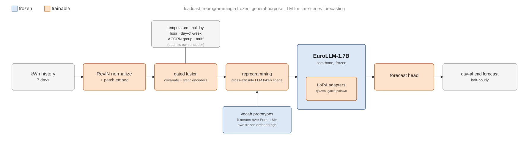
That’s the architecture. In algorithmic form, real PyTorch calls kept:
def forward(batch):
    x ← RevIN.normalize(batch.target)
    patches ← PatchEmbedding(x)
    covariates ← gate(CovariateEncoder(batch.temperature, batch.holiday, batch.calendar))
    static ← gate(StaticEmbed(batch.acorn, batch.tariff))
    tokens ← patches + covariates + static

    prototypes ← kmeans(LLM.embedding_matrix)          # fixed, precomputed once
    reprogrammed ← CrossAttention(query=tokens, key=value=prototypes)

    hidden ← FrozenLLM_with_LoRA(reprogrammed)
    forecast ← ForecastHead(hidden)
    return RevIN.denormalize(forecast)
Training optimizes it, same algorithmic form:
for epoch in epochs:
    for batch in train_loader:              # batch.target: history, batch.future: ground truth
        forecast ← forward(batch)
        loss ← huber_loss(normalize(forecast), normalize(batch.future))   # RevIN-normalized
        loss.backward()
        clip_grad_norm_(trainable_params)
        optimizer.step(); scheduler.step()

    mase ← evaluate_holdout(forward)
    save_checkpoint(run_name)
    if mase < best_mase: save_checkpoint(run_name + "_best")
RevIN, reversible instance normalization, rescales each window by its own mean and standard deviation before the model ever sees it, then undoes that rescaling on the output. The loss is computed in that normalized space rather than raw kWh, so every household’s gradient contribution stays on the same scale. It uses Huber loss instead of MSE, keeping one noisy window’s effect on the whole batch’s loss bounded.
The split is by household rather than by time. 900 training households, 30 held out. Stratified by ACORN group (a UK classification of households by socioeconomic and lifestyle type) and tariff type, split once with a fixed seed rather than k-fold cross-validated.
Each forecast uses 7 days of history to predict the next day, half-hour by half-hour. Evaluation runs on a fixed window stride across the holdout set: 5,944 windows total. Training took about 100 minutes, on a single M4 MacBook Pro.
MASE, mean absolute scaled error, scores a forecast against a naive same-time-yesterday repeat: a MASE of 0.8 means the average error is 80% the size of that naive baseline’s, not an absolute 0.8 kWh. Below 1.0 means beating the baseline, but the margins here are modest, not dramatic: even Chronos, the best of everything tested, is still making about 75% of naive’s error. That says as much about how strong the baseline is as about the models: a lot of a single household’s half-hourly demand really is routine, so “the same time yesterday” is a harder target to beat than it looks. The table below also reports MAE in kWh directly, for a concrete sense of scale.
Overfitting is checked against a same-size sample of training households: MASE 0.844, close to the holdout’s 0.855, too small a gap for serious overfitting. Checkpointing tracks holdout MASE every epoch and keeps the best one, since that peak doesn’t always land on the last epoch. Here it peaked at epoch 6 of 8.
The comparison spans a tiered ladder of approaches. Seasonal-naive is the baseline. LightGBM is classical ML: a single gradient-boosted-trees model, trained once across all training households on lagged and calendar features. Auto-ARIMA is classical too, but statistical rather than learned: a seasonal order fit per household, refit for every evaluation window. Above that, deep learning trained from scratch on this data: an LSTM and a dilated CNN, both fed the raw sequence directly, sized conventionally for their architecture family rather than parameter-matched to LoadCast. Parameter-matching isolates whether pretraining is earning its keep: hold capacity fixed, and only the approach differs. That wasn’t practical for the LSTM and CNN, though. An LSTM sized to match LoadCast’s parameter count was still stuck in its first epoch after 30+ minutes, against 88 seconds for the equivalently-sized Transformer’s whole epoch: LSTMs process a sequence step by step, so wall-clock cost scales with size far more steeply than a Transformer’s parallel attention does. The CNN’s case is murkier: a parameter-matched version stalled the same way after 15+ minutes for reasons never fully diagnosed, against a 2-minute total run for its smaller replacement. One tier up, a from-scratch Transformer, patch-based like LoadCast, parameter-matched to LoadCast’s own trainable count (19.3M against 18.0M): a modern architecture, initialized entirely from scratch. Chronos (chronos-bolt-small, 48M parameters, T5-based) is modern in a different sense, a genuine time-series foundation model, pretrained at scale, zero-shot. LoadCast is the last rung: fine-tuning a general-purpose LLM pretrained on text rather than time series.
| Method | Category | MASE | MAE (kWh) |
|---|---|---|---|
| Chronos (zero-shot) | Foundation model | 0.755 | 0.092 |
| Scratch Transformer | Modern (from scratch) | 0.809 | 0.100 |
| LSTM | Deep learning | 0.851 | 0.106 |
| LoadCast | Fine-tuned general LLM | 0.855 | 0.106 |
| CNN | Deep learning | 0.860 | 0.108 |
| Auto-ARIMA | Classical (statistical) | 0.981 | 0.118 |
| LightGBM | Classical (ML) | 0.992 | 0.119 |
| Seasonal-naive | Baseline | 1.003 | 0.120 |
Chronos wins, though more narrowly than the ranking alone suggests. Its gap to the next-best method is 0.054 MASE, only slightly larger than the 0.051 MASE spread across everything else in the deep-learning cluster below it. Chronos still leads LoadCast, by about 0.014 kWh per half-hour reading on average. Small on its own, but worth sizing against something real: a typical half-hourly reading across these households averages 0.24 kWh, with genuine spread, some readings barely above zero, others well past 1 kWh. An error of 0.09 to 0.11 kWh, Chronos to LoadCast, is a substantial fraction of that. What it means at grid scale is a different question. Individual households’ errors are largely independent of each other, and independent errors partially cancel when aggregated, the same reason a portfolio’s risk is smaller than any single holding’s. A grid operator forecasting a whole substation would see a smaller relative error than anything in this table, even though it would be built from exactly these imprecise household forecasts. Whether that closes the Chronos-LoadCast gap in any way that matters remains an open question, and the right one to ask before treating either number as decisive on its own. Below Chronos, the picture is flatter than expected. LoadCast, the scratch Transformer, the LSTM, and the CNN all land within that same 0.051 MASE of each other, a tight cluster of everything that’s actually deep learning on this data. LoadCast sits squarely in the middle of it, despite being the only one built on a pretrained backbone, and the only one that took anywhere near as long to train: 100 minutes, against 2 to 12 for the others. Every from-scratch baseline shares LoadCast’s own learning rate and schedule too, tuned for a frozen-backbone-plus-LoRA setup specifically, rather than getting its own hyperparameter search, so a properly-tuned LSTM or Transformer might do better yet. This cluster is a floor for them, with real headroom above it. Every deep-learning method clears the classical toolkit by a real margin, regardless: Auto-ARIMA, LightGBM, and seasonal-naive cluster separately, within 0.03 MASE of each other, essentially tied. The one thing that’s helped LoadCast specifically is training on more households. 150, then 450, then 900. Each step improved holdout MASE a bit further. Whether more data alone would ever separate it from the rest of the deep-learning cluster, or close the gap to Chronos, remains an open question. Every number here also comes from a single training run per method, one seed only, so the exact ranking within a few hundredths of MASE is less certain than it looks. The broad shape, Chronos ahead, everything else clustered, classical trailing, is the part worth trusting.
Covariates change the result only marginally, whether on or off. Checking the trained gates explains why: temperature, holiday, and calendar each start at a small, deliberately gentle contribution, a sigmoid-scaled gate initialized to let through about 12% of the signal, and after the full run, every one of them is still sitting within a couple of percentage points of that same starting value. They stayed near their initial value throughout training. Whether that’s a training-signal problem, a single scalar gate is a narrow channel for gradient to push through, or these covariates are mostly redundant with what the model already infers from recent history, remains an open question.
The table only shows averages. Here’s what six of those held-out households actually look like, forecast window by forecast window:
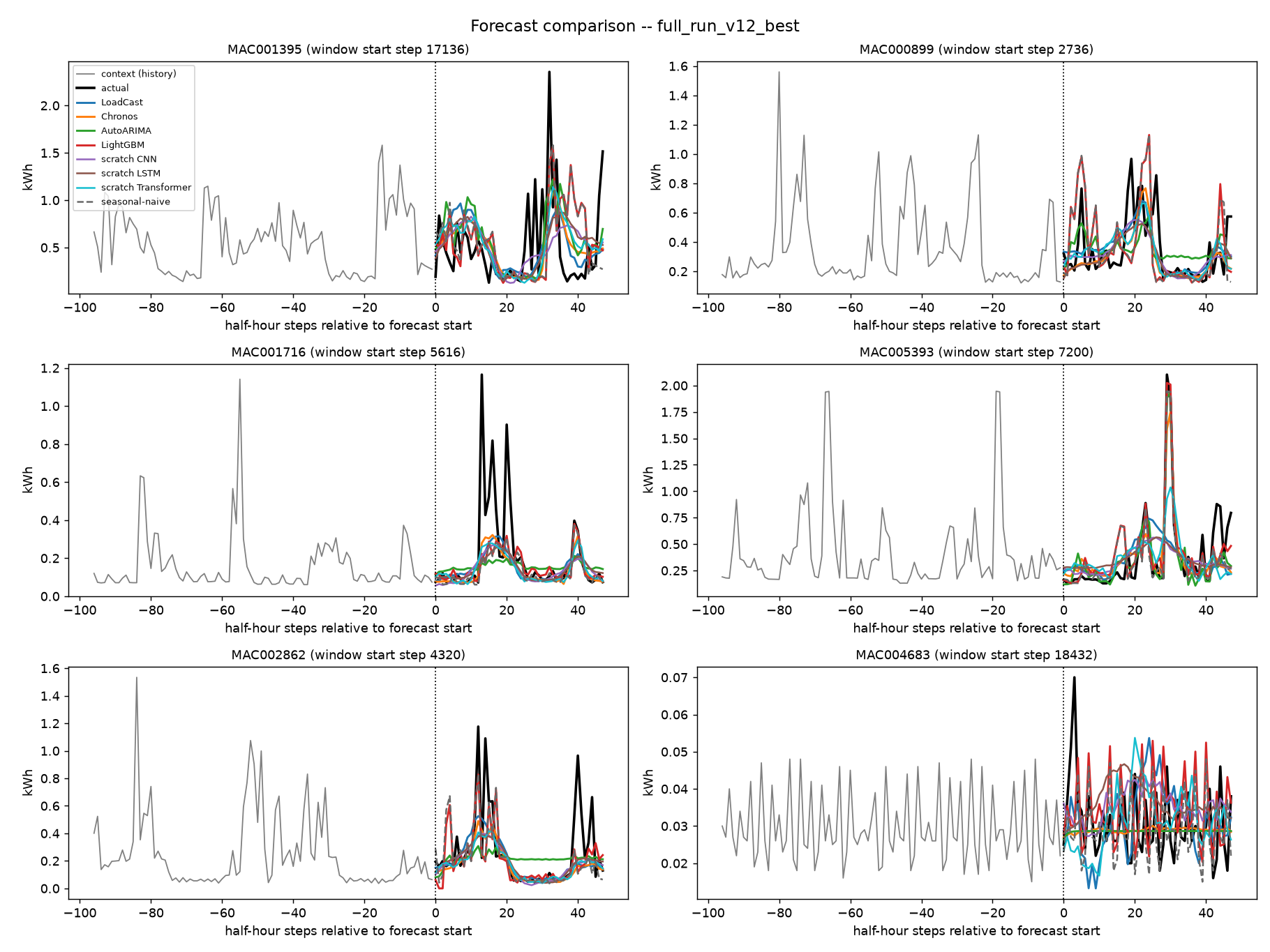
LoadCast and Chronos track closely on most of these. Both smooth over the sharpest spikes in actual demand. The six panels are genuinely different profiles, though. Three households are mostly flat with occasional large spikes, and every method, LoadCast included, misses at least one of those spikes outright, less a modeling gap than genuinely unpredictable behavior. One household’s single spike, by contrast, is caught closely by most methods, including seasonal-naive, suggesting a more routine, learnable pattern behind it, though the scratch LSTM alone flags a false alarm about ten steps early that nothing else shares. On the low-consumption, high-frequency-noise household, every method except Chronos and Auto-ARIMA chases the noise instead of smoothing over it. It’s a tentative, illustrative read across six windows, a reminder that one averaged MASE number hides real variation in how, and when, these methods actually fail.
I tested the language-capability argument directly, in a small way. LoadCast itself can only output numbers: reprogramming loads only a numeric forecast head, so any words about the forecast have to come from somewhere else. Pairing it with a separate, ordinarily instruction-tuned sibling model does work, technically. But the language side is currently weak. Left to reason freely over the numbers, even a well-prompted small instruct model hallucinated readily. A working version needed its role narrowed to paraphrasing a fact computed in advance, checked afterward for invented numbers. An early exercise, with the verdict still to come.
Accuracy is one axis among several here, and on the others the ranking flips. Chronos and seasonal-naive need zero training, ever. Point either at a new household’s recent history and it just works, the same one-shot advantage that makes foundation models attractive regardless of raw accuracy. Auto-ARIMA is the opposite extreme, tied to a single household by construction: a fresh order search and refit for every one. Everything else is a global model instead, applying directly to new households. But each one still needs an initial training pass, and eventually a repeat of it. That costs about 2 minutes for the CNN, 20 for LightGBM, 100 for LoadCast, on this hardware. LoadCast sits at the expensive end, for a result the cheaper alternatives equal anyway. Explainability tells a similar story. Classical methods are interpretable by construction: Auto-ARIMA’s coefficients, LightGBM’s feature importances. The from-scratch deep nets are moderately so; attention over raw patches, LSTM gate dynamics, and CNN receptive fields all have mature interpretability tooling built for them. LoadCast is the least legible of any of them. Its forecast arrives via reprogramming into a frozen 1.7B-parameter LLM’s embedding space, a genuinely more exotic mechanism, with far less interpretability tooling built for it than any simpler architecture here. That’s a qualitative judgment on my part, offered alongside the measured numbers above.
So the general-purpose LLM still trails, and the case against it now extends beyond accuracy. LoadCast blends into a cluster of from-scratch deep-learning alternatives, an LSTM, a CNN, a plain Transformer, that took a fraction of the training time and, in two of three cases, a fraction of the parameters too. It’s also the most expensive of everything tested to retrain, and the least explainable. On accuracy, cost, and explainability alike, the alternatives come out ahead of whatever EuroLLM’s pretrained weights contribute here. Two questions stay open regardless: whether reprogramming would ever earn back that gap with more data or a proper hyperparameter search of its own, and whether a reprogrammed LLM can genuinely talk about what it forecasts, tested above in a small way and still early. The second one is the more interesting bet. It’s the one thing here that a purpose-built model, however cheap and however accurate, was never built to do.
Coming back to that: mostly, once aggregated, a single household’s forecast error doesn’t matter much, the same portfolio effect that makes a grid operator’s job easier than any one forecast would suggest. It matters more directly downstream of that. A battery scheduler, a demand-response programme, a peer-to-peer market like MAS4TE: all of them dispatch against a forecast, and a bad one means charging a battery at the wrong hour or mispricing a trade. As more of the grid’s flexibility moves down to the household level, batteries, EVs, solar, that’s where forecast accuracy actually earns its keep.
AI attribution:

Human-AI blend: AI wrote the scratch Transformer/LSTM/CNN baseline code and polished this post’s prose. I directed and reviewed both. The code specifically, I trusted as given. Model: Claude Sonnet 5, Anthropic. Statement via the AI Attribution Toolkit.